The system of linear equations is called joint if mti. How to find a general and particular solution to a system of linear equations

We continue to deal with systems of linear equations. So far, we have considered systems that have a unique solution. Such systems can be solved in any way: substitution method("school") by Cramer's formulas, matrix method, Gauss method. However, two more cases are widespread in practice when:

1) the system is inconsistent (has no solutions);

2) the system has infinitely many solutions.

For these systems, the most universal of all solution methods is used - Gauss method. In fact, the “school” way will also lead to the answer, but in higher mathematics It is customary to use the Gaussian method of successive elimination of unknowns. Those who are not familiar with the Gauss method algorithm, please study the lesson first Gauss method

The elementary matrix transformations themselves are exactly the same, the difference will be in the end of the solution. First, consider a couple of examples where the system has no solutions (inconsistent).

Example 1

What immediately catches your eye in this system? The number of equations is less than the number of variables. There is a theorem that says: “If the number of equations in the system less quantity variables, then the system is either inconsistent or has infinitely many solutions. And it remains only to find out.

The beginning of the solution is quite ordinary - we write the extended matrix of the system and, using elementary transformations, we bring it to a stepwise form:

(one). On the upper left step, we need to get (+1) or (-1). There are no such numbers in the first column, so rearranging the rows will not work. The unit will have to be organized independently, and this can be done in several ways. We did so. To the first line we add the third line, multiplied by (-1).

(2). Now we get two zeros in the first column. To the second line, add the first line, multiplied by 3. To the third line, add the first, multiplied by 5.

(3). After the transformation is done, it is always advisable to see if it is possible to simplify the resulting strings? Can. We divide the second line by 2, at the same time getting the desired one (-1) on the second step. Divide the third line by (-3).

(4). Add the second line to the third line. Probably, everyone paid attention to the bad line, which turned out as a result of elementary transformations:

. It is clear that this cannot be so.

Indeed, we rewrite the resulting matrix

back to the system of linear equations:

If as a result of elementary transformations a string of the form , whereλ is a non-zero number, then the system is inconsistent (has no solutions).

How to record the end of a task? You need to write down the phrase:

“As a result of elementary transformations, a string of the form is obtained, where λ ≠ 0 ". Answer: "The system has no solutions (inconsistent)."

Please note that in this case there is no reverse move of the Gaussian algorithm, there are no solutions and there is simply nothing to find.

Example 2

Solve a system of linear equations

This is a do-it-yourself example. Complete Solution and the answer at the end of the lesson.

Again, we remind you that your solution path may differ from our solution path, the Gauss method does not set an unambiguous algorithm, you must guess the procedure and the actions themselves in each case independently.

Another one technical feature solutions: elementary transformations can be stopped At once, as soon as a line like , where λ ≠ 0 . Consider conditional example: suppose that after the first transformation we get a matrix

This matrix has not yet been reduced to a stepped form, but there is no need for further elementary transformations, since a line of the form has appeared, where λ ≠ 0 . It should be immediately answered that the system is incompatible.

When a system of linear equations has no solutions, this is almost a gift to the student, due to the fact that a short solution is obtained, sometimes literally in 2-3 steps. But everything in this world is balanced, and the problem in which the system has infinitely many solutions is just longer.

Example 3:

Solve a system of linear equations

There are 4 equations and 4 unknowns, so the system can either have a single solution, or have no solutions, or have an infinite number of solutions. Whatever it was, but the Gauss method in any case will lead us to the answer. This is its versatility.

The beginning is again standard. We write the extended matrix of the system and, using elementary transformations, bring it to a step form:

That's all, and you were afraid.

(one). Please note that all the numbers in the first column are divisible by 2, so on the upper left step we are also satisfied with a deuce. To the second line we add the first line, multiplied by (-4). To the third line we add the first line, multiplied by (-2). To the fourth line we add the first line, multiplied by (-1).

Attention! Many may be tempted from the fourth line subtract first line. This can be done, but it is not necessary, experience shows that the probability of an error in calculations increases several times. We just add: to the fourth line we add the first line, multiplied by (-1) - exactly!

(2). The last three lines are proportional, two of them can be deleted. Here again it is necessary to show increased attention, but are the lines really proportional? For reinsurance, it will not be superfluous to multiply the second row by (-1), and divide the fourth row by 2, resulting in three identical rows. And only after that remove two of them. As a result of elementary transformations, the extended matrix of the system is reduced to a stepped form:

When completing a task in a notebook, it is advisable to make the same notes in pencil for clarity.

We rewrite the corresponding system of equations:

The “usual” only solution of the system does not smell here. Bad line where λ ≠ 0, also no. Hence, this is the third remaining case - the system has infinitely many solutions.

The infinite set of solutions of the system is briefly written in the form of the so-called general system solution.

We will find the general solution of the system using the reverse motion of the Gauss method. For systems of equations with an infinite set of solutions, new concepts appear: "basic variables" and "free variables". First, let's define what variables we have basic, and what variables - free. It is not necessary to explain in detail the terms of linear algebra, it is enough to remember that there are such basis variables and free variables.

Basic variables always "sit" strictly on the steps of the matrix. In this example, the base variables are x 1 and x 3 .

Free variables are everything remaining variables that did not get a step. In our case, there are two: x 2 and x 4 - free variables.

Now you need allbasis variables express only throughfree variables. The reverse move of the Gaussian algorithm traditionally works from the bottom up. From the second equation of the system, we express the basic variable x 3:

Now look at the first equation: . First, we substitute the found expression into it:

It remains to express the basic variable x 1 through free variables x 2 and x 4:

The result is what you need - all basis variables ( x 1 and x 3) expressed only through free variables ( x 2 and x 4):

Actually, the general solution is ready:

How to write down the general solution? First of all, free variables are written into the general solution “on their own” and strictly in their places. In this case, the free variables x 2 and x 4 should be written in the second and fourth positions:

The resulting expressions for the basic variables and obviously needs to be written in the first and third positions:

From the general solution of the system, one can find infinitely many private decisions. It's very simple. free variables x 2 and x 4 are called so because they can be given any final values. The most popular values are zero values, since this is the easiest way to obtain a particular solution.

Substituting ( x 2 = 0; x 4 = 0) into the general solution, we get one of the particular solutions:

, or is a particular solution corresponding to free variables with values ( x 2 = 0; x 4 = 0).

Ones are another sweet couple, let's substitute ( x 2 = 1 and x 4 = 1) into the general solution:

, i.e. (-1; 1; 1; 1) is another particular solution.

It is easy to see that the system of equations has infinitely many solutions since we can give free variables any values.

Each a particular solution must satisfy to each system equation. This is the basis for a “quick” check of the correctness of the solution. Take, for example, a particular solution (-1; 1; 1; 1) and substitute it into the left side of each equation in the original system:

Everything has to come together. And with any particular solution you get, everything should also converge.

Strictly speaking, the verification of a particular solution sometimes deceives, i.e. some particular solution can satisfy each equation of the system, and the general solution itself is actually found incorrectly. Therefore, first of all, the verification of the general solution is more thorough and reliable.

How to check the resulting general solution ?

It's not difficult, but it requires quite a long transformation. We need to take expressions basic variables, in this case and , and substitute them into the left side of each equation of the system.

To the left side of the first equation of the system:

The right side of the original first equation of the system is obtained.

To the left side of the second equation of the system:

The right side of the original second equation of the system is obtained.

And further - to the left parts of the third and fourth equations of the system. This check is longer, but it guarantees the 100% correctness of the overall solution. In addition, in some tasks it is required to check the general solution.

Example 4:

Solve the system using the Gauss method. Find a general solution and two private ones. Check the overall solution.

This is a do-it-yourself example. Here, by the way, again the number of equations is less than the number of unknowns, which means that it is immediately clear that the system will either be inconsistent or have an infinite number of solutions.

Example 5:

Solve a system of linear equations. If the system has infinitely many solutions, find two particular solutions and check the general solution

Decision: Let us write down the extended matrix of the system and, with the help of elementary transformations, bring it to a stepped form:

(one). Add the first line to the second line. To the third line we add the first line multiplied by 2. To the fourth line we add the first line multiplied by 3.

(2). To the third line we add the second line, multiplied by (-5). To the fourth line we add the second line, multiplied by (-7).

(3). The third and fourth lines are the same, we delete one of them. Here is such a beauty:

Basis variables sit on steps, so they are base variables.

There is only one free variable, which did not get a step: .

(4). Reverse move. We express the basic variables in terms of the free variable:

From the third equation:

Consider the second equation and substitute the found expression into it:

, , ,

Consider the first equation and substitute the found expressions and into it:

Thus, the general solution with one free variable x 4:

Once again, how did it happen? free variable x 4 sits alone in its rightful fourth place. The resulting expressions for the basic variables , , are also in their places.

Let us immediately check the general solution.

We substitute the basic variables , , into the left side of each equation of the system:

The corresponding right-hand sides of the equations are obtained, thus, the correct general solution is found.

Now from the found general solution we get two particular solutions. All variables are expressed here through a single free variable x 4 . You don't need to break your head.

Let be x 4 = 0, then is the first particular solution.

Let be x 4 = 1, then is another particular solution.

Answer: Common decision: . Private Solutions:

and .

Example 6:

Find the general solution of the system of linear equations.

We have already checked the general solution, the answer can be trusted. Your course of action may differ from our course of action. The main thing is that the general solutions coincide. Probably, many people noticed an unpleasant moment in the solutions: very often, during the reverse course of the Gauss method, we had to fiddle with ordinary fractions. In practice, this is true, cases where there are no fractions are much less common. Be prepared mentally, and most importantly, technically.

Let us dwell on the features of the solution that were not found in the solved examples. The general solution of the system may sometimes include a constant (or constants).

For example, the general solution: . Here one of the basic variables is equal to a constant number: . There is nothing exotic in this, it happens. Obviously, in this case, any particular solution will contain a five in the first position.

Rarely, but there are systems in which the number of equations is greater than the number of variables. However, the Gauss method works under the most severe conditions. You should calmly bring the extended matrix of the system to a stepped form according to the standard algorithm. Such a system may be inconsistent, may have infinitely many solutions, and, oddly enough, may have a unique solution.

We repeat in our advice - in order to feel comfortable when solving a system using the Gauss method, you should fill your hand and solve at least a dozen systems.

Solutions and answers:

Example 2:

Decision:Let us write down the extended matrix of the system and, using elementary transformations, bring it to a stepped form.

Performed elementary transformations:

(1) The first and third lines have been swapped.

(2) The first line was added to the second line, multiplied by (-6). The first line was added to the third line, multiplied by (-7).

(3) The second line was added to the third line, multiplied by (-1).

As a result of elementary transformations, a string of the form, where λ ≠ 0 .So the system is inconsistent.Answer: there are no solutions.

Example 4:

Decision:We write the extended matrix of the system and, using elementary transformations, bring it to a step form:

Conversions performed:

(one). The first line multiplied by 2 was added to the second line. The first line multiplied by 3 was added to the third line.

There is no unit for the second step , and transformation (2) is aimed at obtaining it.

(2). The second line was added to the third line, multiplied by -3.

(3). The second and third rows were swapped (the resulting -1 was moved to the second step)

(4). The second line was added to the third line, multiplied by 3.

(5). The sign of the first two lines was changed (multiplied by -1), the third line was divided by 14.

Reverse move:

(one). Here are the basic variables (which are on steps), and are free variables (who did not get the step).

(2). We express the basic variables in terms of free variables:

From the third equation: .

(3). Consider the second equation:, particular solutions:

Answer: Common decision:

Complex numbers

In this section, we will introduce the concept complex number, consider algebraic, trigonometric and show form complex number. We will also learn how to perform operations with complex numbers: addition, subtraction, multiplication, division, exponentiation and root extraction.

To master complex numbers, you do not need any special knowledge from the course of higher mathematics, and the material is available even to a schoolboy. It is enough to be able to perform algebraic operations with "ordinary" numbers, and remember trigonometry.

First, let's remember the "ordinary" Numbers. In mathematics they are called many real numbers and are marked with the letter R, or R (thick). All real numbers sit on the familiar number line:

The company of real numbers is very colorful - here are whole numbers, and fractions, and irrational numbers. In this case, each point of the numerical axis necessarily corresponds to some real number.

Systems m linear equations with n unknown.
Solving a system of linear equations is such a set of numbers ( x 1 , x 2 , …, x n), substituting which into each of the equations of the system, the correct equality is obtained.
where a ij , i = 1, …, m; j = 1, …, n are the coefficients of the system;
b i , i = 1, …, m- free members;
x j , j = 1, …, n- unknown.
The above system can be written in matrix form: A X = B,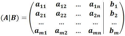

where ( A|B) is the main matrix of the system;
A— extended matrix of the system;
X— column of unknowns;
B is a column of free members.
If the matrix B is not a null matrix ∅, then this system of linear equations is called inhomogeneous.
If the matrix B= ∅, then this system of linear equations is called homogeneous. A homogeneous system always has a zero (trivial) solution: x 1 \u003d x 2 \u003d ..., x n \u003d 0.
Joint system of linear equations is a system of linear equations that has a solution.
Inconsistent system of linear equations is a system of linear equations that has no solution.
Certain system of linear equations is a system of linear equations that has a unique solution.
Indefinite system of linear equations is a system of linear equations that has an infinite number of solutions.
Systems of n linear equations with n unknowns
If the number of unknowns is equal to the number of equations, then the matrix is square. The matrix determinant is called the main determinant of the system of linear equations and is denoted by the symbol Δ.
Cramer method for solving systems n linear equations with n unknown.
Cramer's rule.
If the main determinant of the system of linear equations is not zero, then the system is consistent and defined, and the unique solution is calculated by the Cramer formulas:
where Δ i are the determinants obtained from the main determinant of the system Δ by replacing i th column to the column of free members. .
Systems of m linear equations with n unknowns
Kronecker-Cappelli theorem.

In order for this system of linear equations to be consistent, it is necessary and sufficient that the rank of the matrix of the system be equal to the rank of the extended matrix of the system, rank(Α) = rank(Α|B).
If a rang(Α) ≠ rang(Α|B), then the system obviously has no solutions.
If rank(Α) = rank(Α|B), then two cases are possible:
1) rang(Α) = n(to the number of unknowns) - the solution is unique and can be obtained by Cramer's formulas;
2) rank(Α)< n − there are infinitely many solutions.
Gauss method for solving systems of linear equations

Let's compose the augmented matrix ( A|B) of the given system of coefficients at the unknown and right-hand sides.
The Gaussian method or the elimination of unknowns method consists in reducing the augmented matrix ( A|B) with the help of elementary transformations over its rows to a diagonal form (to an upper triangular form). Returning to the system of equations, all unknowns are determined.
Elementary transformations on strings include the following:
1) swapping two lines;
2) multiplying a string by a number other than 0;
3) adding to the string another string multiplied by an arbitrary number;
4) discarding a null string.
An extended matrix reduced to a diagonal form corresponds to a linear system equivalent to the given one, the solution of which does not cause difficulties. .
System of homogeneous linear equations.
The homogeneous system has the form:

it corresponds to the matrix equation A X = 0.
1) A homogeneous system is always consistent, since r(A) = r(A|B), there is always a zero solution (0, 0, …, 0).
2) For a homogeneous system to have a nonzero solution, it is necessary and sufficient that r = r(A)< n , which is equivalent to Δ = 0.
3) If r< n , then Δ = 0, then there are free unknowns c 1 , c 2 , …, c n-r, the system has nontrivial solutions, and there are infinitely many of them.
4) General solution X at r< n can be written in matrix form as follows:
X \u003d c 1 X 1 + c 2 X 2 + ... + c n-r X n-r,
where are the solutions X 1 , X 2 , …, X n-r form a fundamental system of solutions.
5) The fundamental system of solutions can be obtained from the general solution of the homogeneous system:

,
if we sequentially assume the values of the parameters to be (1, 0, …, 0), (0, 1, …, 0), …, (0, 0, …, 1).
Decomposition of the general solution in terms of the fundamental system of solutions is a record of the general solution as a linear combination of solutions belonging to the fundamental system.
Theorem. For a system of linear homogeneous equations to have a nonzero solution, it is necessary and sufficient that Δ ≠ 0.
So, if the determinant is Δ ≠ 0, then the system has a unique solution.
If Δ ≠ 0, then the system of linear homogeneous equations has an infinite number of solutions.
Theorem. For a homogeneous system to have a nonzero solution, it is necessary and sufficient that r(A)< n .
Proof:
1) r can't be more n(matrix rank does not exceed the number of columns or rows);
2) r< n , because if r=n, then the main determinant of the system Δ ≠ 0, and, according to Cramer's formulas, there is a unique trivial solution x 1 \u003d x 2 \u003d ... \u003d x n \u003d 0, which contradicts the condition. Means, r(A)< n .
Consequence. In order for a homogeneous system n linear equations with n unknowns has a nonzero solution, it is necessary and sufficient that Δ = 0.

Service assignment. The online calculator is designed to study a system of linear equations. Usually in the condition of the problem it is required to find general and particular solution of the system. When studying systems of linear equations, the following problems are solved:

whether the system is collaborative;
if the system is consistent, then it is definite or indefinite (the criterion of system compatibility is determined by the theorem);
if the system is defined, then how to find its unique solution (the Cramer method, the inverse matrix method or the Jordan-Gauss method are used);
if the system is indefinite, then how to describe the set of its solutions.

Classification of systems of linear equations

An arbitrary system of linear equations has the form:
a 1 1 x 1 + a 1 2 x 2 + ... + a 1 n x n = b 1
a 2 1 x 1 + a 2 2 x 2 + ... + a 2 n x n = b 2
...................................................
a m 1 x 1 + a m 2 x 2 + ... + a m n x n = b m

Systems of linear inhomogeneous equations (the number of variables is equal to the number of equations, m = n).
Arbitrary systems of linear inhomogeneous equations (m > n or m< n).

Definition. A solution of a system is any set of numbers c 1 ,c 2 ,...,c n , whose substitution into the system instead of the corresponding unknowns turns each equation of the system into an identity.

Definition. Two systems are said to be equivalent if the solution to the first is the solution to the second and vice versa.

Definition. A system that has at least one solution is called joint. A system that does not have any solution is called inconsistent.

Definition. A system with a unique solution is called certain, and having more than one solution is indefinite.

Algorithm for solving systems of linear equations

Find the ranks of the main and extended matrices. If they are not equal, then, by the Kronecker-Capelli theorem, the system is inconsistent, and this is where the study ends.
Let rank(A) = rank(B) . We select the basic minor. In this case, all unknown systems of linear equations are divided into two classes. The unknowns, the coefficients of which are included in the basic minor, are called dependent, and the unknowns, the coefficients of which are not included in the basic minor, are called free. Note that the choice of dependent and free unknowns is not always unique.
We cross out those equations of the system whose coefficients were not included in the basic minor, since they are consequences of the rest (according to the basic minor theorem).
The terms of the equations containing free unknowns will be transferred to the right side. As a result, we obtain a system of r equations with r unknowns, equivalent to the given one, the determinant of which is different from zero.
The resulting system is solved in one of the following ways: the Cramer method, the inverse matrix method, or the Jordan-Gauss method. Relations are found that express the dependent variables in terms of the free ones.

System of m linear equations with n unknowns called a system of the form

where aij and b i (i=1,…,m; b=1,…,n) are some known numbers, and x 1 ,…,x n- unknown. In the notation of the coefficients aij first index i denotes the number of the equation, and the second j is the number of the unknown at which this coefficient stands.

The coefficients for the unknowns will be written in the form of a matrix , which we will call system matrix.

The numbers on the right sides of the equations b 1 ,…,b m called free members.

Aggregate n numbers c 1 ,…,c n called decision of this system, if each equation of the system becomes an equality after substituting numbers into it c 1 ,…,c n instead of the corresponding unknowns x 1 ,…,x n.

Our task will be to find solutions to the system. In this case, three situations may arise:

A system of linear equations that has at least one solution is called joint. Otherwise, i.e. if the system has no solutions, then it is called incompatible.

Consider ways to find solutions to the system.

MATRIX METHOD FOR SOLVING SYSTEMS OF LINEAR EQUATIONS

Matrices make it possible to briefly write down a system of linear equations. Let a system of 3 equations with three unknowns be given:

Consider the matrix of the system and matrix columns of unknown and free members

Let's find the product

those. as a result of the product, we obtain the left-hand sides of the equations of this system. Then using the definition of matrix equality this system can be written in the form

or shorter A∙X=B.

Here matrices A and B are known, and the matrix X unknown. She needs to be found, because. its elements are the solution of this system. This equation is called matrix equation.

Let the matrix determinant be different from zero | A| ≠ 0. Then the matrix equation is solved as follows. Multiply both sides of the equation on the left by the matrix A-1, the inverse of the matrix A: . Insofar as A -1 A = E and E∙X=X, then we obtain the solution of the matrix equation in the form X = A -1 B .

Note that since the inverse matrix can only be found for square matrices, the matrix method can only solve those systems in which the number of equations is the same as the number of unknowns. However, the matrix notation of the system is also possible in the case when the number of equations is not equal to the number of unknowns, then the matrix A is not square and therefore it is impossible to find a solution to the system in the form X = A -1 B.

Examples. Solve systems of equations.

CRAMER'S RULE

Consider a system of 3 linear equations with three unknowns:

Third-order determinant corresponding to the matrix of the system, i.e. composed of coefficients at unknowns,

called system determinant.

We compose three more determinants as follows: we replace successively 1, 2 and 3 columns in the determinant D with a column of free terms

Then we can prove the following result.

Theorem (Cramer's rule). If the determinant of the system is Δ ≠ 0, then the system under consideration has one and only one solution, and

Proof. So, consider a system of 3 equations with three unknowns. Multiply the 1st equation of the system by the algebraic complement A 11 element a 11, 2nd equation - on A21 and 3rd - on A 31:

Let's add these equations:

Consider each of the brackets and the right side of this equation. By the theorem on the expansion of the determinant in terms of the elements of the 1st column

Similarly, it can be shown that and .

Finally, it is easy to see that

Thus, we get the equality: .

Hence, .

The equalities and are derived similarly, whence the assertion of the theorem follows.

Thus, we note that if the determinant of the system is Δ ≠ 0, then the system has a unique solution and vice versa. If the determinant of the system is equal to zero, then the system either has an infinite set of solutions or has no solutions, i.e. incompatible.

Examples. Solve a system of equations

GAUSS METHOD

The previously considered methods can be used to solve only those systems in which the number of equations coincides with the number of unknowns, and the determinant of the system must be different from zero. The Gaussian method is more universal and is suitable for systems with any number of equations. It consists in the successive elimination of unknowns from the equations of the system.

Consider again a system of three equations with three unknowns:

We leave the first equation unchanged, and from the 2nd and 3rd we exclude the terms containing x 1. To do this, we divide the second equation by a 21 and multiply by - a 11 and then add with the 1st equation. Similarly, we divide the third equation into a 31 and multiply by - a 11 and then add it to the first one. As a result, the original system will take the form:

Now, from the last equation, we eliminate the term containing x2. To do this, divide the third equation by , multiply by and add it to the second. Then we will have a system of equations:

Hence from the last equation it is easy to find x 3, then from the 2nd equation x2 and finally from the 1st - x 1.

When using the Gaussian method, the equations can be interchanged if necessary.

Often instead of writing new system equations are limited to writing out the extended matrix of the system:

and then bring it to a triangular or diagonal form using elementary transformations.

To elementary transformations matrices include the following transformations:

permutation of rows or columns;
multiplying a string by a non-zero number;
adding to one line other lines.

Examples: Solve systems of equations using the Gauss method.

Thus, the system has an infinite number of solutions.

Systems of equations are widely used in the economic industry in the mathematical modeling of various processes. For example, when solving problems of production management and planning, logistics routes (transport problem) or equipment placement.

Equation systems are used not only in the field of mathematics, but also in physics, chemistry and biology, when solving problems of finding the population size.

A system of linear equations is a term for two or more equations with several variables for which it is necessary to find a common solution. Such a sequence of numbers for which all equations become true equalities or prove that the sequence does not exist.

Linear Equation

Equations of the form ax+by=c are called linear. The designations x, y are the unknowns, the value of which must be found, b, a are the coefficients of the variables, c is the free term of the equation.
Solving the equation by plotting its graph will look like a straight line, all points of which are the solution of the polynomial.

Types of systems of linear equations

The simplest are examples of systems of linear equations with two variables X and Y.

F1(x, y) = 0 and F2(x, y) = 0, where F1,2 are functions and (x, y) are function variables.

Solve a system of equations - it means to find such values (x, y) at which the system turns into a true equality or establish that suitable values x and y do not exist.

A pair of values (x, y), written as point coordinates, is called a solution to a system of linear equations.

If the systems have one common solution or there is no solution, they are called equivalent.

Homogeneous systems of linear equations are systems whose right side is equal to zero. If the right part after the "equal" sign has a value or is expressed by a function, such a system is not homogeneous.

The number of variables can be much more than two, then we should talk about an example of a system of linear equations with three variables or more.

Faced with systems, schoolchildren assume that the number of equations must necessarily coincide with the number of unknowns, but this is not so. The number of equations in the system does not depend on the variables, there can be an arbitrarily large number of them.

Simple and complex methods for solving systems of equations

There is no general analytical way to solve such systems, all methods are based on numerical solutions. The school mathematics course describes in detail such methods as permutation, algebraic addition, substitution, as well as the graphical and matrix method, the solution by the Gauss method.

The main task in teaching methods of solving is to teach how to correctly analyze the system and find optimal algorithm solutions for each example. The main thing is not to memorize a system of rules and actions for each method, but to understand the principles of applying a particular method.

Solving examples of systems of linear equations of the 7th class of the program secondary school quite simple and explained in great detail. In any textbook on mathematics, this section is given enough attention. The solution of examples of systems of linear equations by the method of Gauss and Cramer is studied in more detail in the first courses of higher educational institutions.

Solution of systems by the substitution method

The actions of the substitution method are aimed at expressing the value of one variable through the second. The expression is substituted into the remaining equation, then it is reduced to a single variable form. The action is repeated depending on the number of unknowns in the system

Let's give an example of a system of linear equations of the 7th class by the substitution method:

As can be seen from the example, the variable x was expressed through F(X) = 7 + Y. The resulting expression, substituted into the 2nd equation of the system in place of X, helped to obtain one variable Y in the 2nd equation. The solution of this example does not cause difficulties and allows you to get the Y value. The last step is to check the obtained values.

It is not always possible to solve an example of a system of linear equations by substitution. The equations can be complex and the expression of the variable in terms of the second unknown will be too cumbersome for further calculations. When there are more than 3 unknowns in the system, the substitution solution is also impractical.

Solution of an example of a system of linear inhomogeneous equations:

Solution using algebraic addition

When searching for a solution to systems by the addition method, term-by-term addition and multiplication of equations by various numbers. The ultimate goal of mathematical operations is an equation with one variable.

Applications of this method require practice and observation. It is not easy to solve a system of linear equations using the addition method with the number of variables 3 or more. Algebraic addition is useful when the equations contain fractions and decimal numbers.

Solution action algorithm:

Multiply both sides of the equation by some number. As a result arithmetic operation one of the coefficients of the variable must become equal to 1.
Add the resulting expression term by term and find one of the unknowns.
Substitute the resulting value into the 2nd equation of the system to find the remaining variable.

Solution method by introducing a new variable

A new variable can be introduced if the system needs to find a solution for no more than two equations, the number of unknowns should also be no more than two.

The method is used to simplify one of the equations by introducing a new variable. The new equation is solved with respect to the entered unknown, and the resulting value is used to determine the original variable.

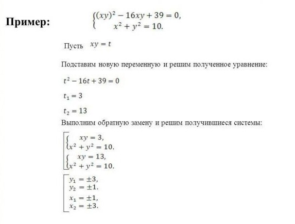
The example shows that by introducing a new variable t, it was possible to reduce the 1st equation of the system to the standard square trinomial. You can solve a polynomial by finding the discriminant.

It is necessary to find the value of the discriminant by well-known formula: D = b2 - 4*a*c, where D is the desired discriminant, b, a, c are the multipliers of the polynomial. In the given example, a=1, b=16, c=39, hence D=100. If the discriminant is greater than zero, then there are two solutions: t = -b±√D / 2*a, if the discriminant is less than zero, then there is only one solution: x= -b / 2*a.

The solution for the resulting systems is found by the addition method.

A visual method for solving systems

Suitable for systems with 3 equations. The method consists in plotting graphs of each equation included in the system on the coordinate axis. The coordinates of the points of intersection of the curves will be the general solution of the system.

The graphic method has a number of nuances. Consider several examples of solving systems of linear equations in a visual way.

As can be seen from the example, two points were constructed for each line, the values of the variable x were chosen arbitrarily: 0 and 3. Based on the values of x, the values for y were found: 3 and 0. Points with coordinates (0, 3) and (3, 0) were marked on the graph and connected by a line.

The steps must be repeated for the second equation. The point of intersection of the lines is the solution of the system.

In the following example, it is required to find a graphical solution to the system of linear equations: 0.5x-y+2=0 and 0.5x-y-1=0.

As can be seen from the example, the system has no solution, because the graphs are parallel and do not intersect along their entire length.

The systems from Examples 2 and 3 are similar, but when constructed, it becomes obvious that their solutions are different. It should be remembered that it is not always possible to say whether the system has a solution or not, it is always necessary to build a graph.

Matrix and its varieties

Matrices are used to briefly write down a system of linear equations. A matrix is a special type of table filled with numbers. n*m has n - rows and m - columns.

A matrix is square when the number of columns and rows is equal. A matrix-vector is a single-column matrix with an infinitely possible number of rows. A matrix with units along one of the diagonals and other zero elements is called identity.

An inverse matrix is such a matrix, when multiplied by which the original one turns into a unit one, such a matrix exists only for the original square one.

Rules for transforming a system of equations into a matrix

With regard to systems of equations, the coefficients and free members of the equations are written as numbers of the matrix, one equation is one row of the matrix.

A matrix row is called non-zero if at least one element of the row is not equal to zero. Therefore, if in any of the equations the number of variables differs, then it is necessary to enter zero in place of the missing unknown.

The columns of the matrix must strictly correspond to the variables. This means that the coefficients of the variable x can only be written in one column, for example the first, the coefficient of the unknown y - only in the second.

When multiplying a matrix, all matrix elements are sequentially multiplied by a number.

Options for finding the inverse matrix

The formula for finding the inverse matrix is quite simple: K -1 = 1 / |K|, where K -1 is the inverse matrix and |K| - matrix determinant. |K| must not be equal to zero, then the system has a solution.

The determinant is easily calculated for a two-by-two matrix, it is only necessary to multiply the elements diagonally by each other. For the "three by three" option, there is a formula |K|=a 1 b 2 c 3 + a 1 b 3 c 2 + a 3 b 1 c 2 + a 2 b 3 c 1 + a 2 b 1 c 3 + a 3 b 2 c 1 . You can use the formula, or you can remember that you need to take one element from each row and each column so that the column and row numbers of the elements do not repeat in the product.

Solution of examples of systems of linear equations by the matrix method

The matrix method of finding a solution makes it possible to reduce cumbersome notations when solving systems with large quantity variables and equations.

In the example, a nm are the coefficients of the equations, the matrix is a vector x n are the variables, and b n are the free terms.

Solution of systems by the Gauss method

In higher mathematics, the Gauss method is studied together with the Cramer method, and the process of finding a solution to systems is called the Gauss-Cramer solution method. These methods are used to find the variables of systems with a large number of linear equations.

The Gaussian method is very similar to substitution and algebraic addition solutions, but is more systematic. In the school course, the Gaussian solution is used for systems of 3 and 4 equations. The purpose of the method is to bring the system to the form of an inverted trapezoid. By algebraic transformations and substitutions, the value of one variable is found in one of the equations of the system. The second equation is an expression with 2 unknowns, and 3 and 4 - with 3 and 4 variables, respectively.

After bringing the system to the described form, the further solution is reduced to the sequential substitution of known variables into the equations of the system.

In school textbooks for grade 7, an example of a Gaussian solution is described as follows:

As can be seen from the example, at step (3) two equations were obtained 3x 3 -2x 4 =11 and 3x 3 +2x 4 =7. The solution of any of the equations will allow you to find out one of the variables x n.

Theorem 5, which is mentioned in the text, says that if one of the equations of the system is replaced by an equivalent one, then the resulting system will also be equivalent to the original one.

The Gauss method is difficult for students to understand high school, but is one of the most interesting ways to develop the ingenuity of children enrolled in the advanced study program in math and physics classes.

For ease of recording calculations, it is customary to do the following:

Equation coefficients and free terms are written in the form of a matrix, where each row of the matrix corresponds to one of the equations of the system. separates the left side of the equation from the right side. Roman numerals denote the numbers of equations in the system.

First, they write down the matrix with which to work, then all the actions carried out with one of the rows. The resulting matrix is written after the "arrow" sign and continue to perform the necessary algebraic operations until the result is achieved.

As a result, a matrix should be obtained in which one of the diagonals is 1, and all other coefficients are equal to zero, that is, the matrix is reduced to a single form. We must not forget to make calculations with the numbers of both sides of the equation.

This notation is less cumbersome and allows you not to be distracted by listing numerous unknowns.

The free application of any method of solution will require care and a certain amount of experience. Not all methods are applied. Some ways of finding solutions are more preferable in a particular area of human activity, while others exist for the purpose of learning.