Demand. Demand functions
The process of exchanging goods in a competitive market has its own laws. They are found in the peculiarities of the economic response of market participants to the ratio of the quantity of exchanged goods and their prices. Thus, one of the most important laws "governing" the process of commodity exchange and pricing in a competitive market is the law of demand.
Demand is the quantity of a good that buyers are willing and able to purchase in a given period of time at all possible prices for that good.
In market conditions, the so-called law of demand, which can be expressed as follows. Ceteris paribus, the higher the demand for a product, the lower the price of this product, and vice versa, the higher the price, the lower the demand for the product. The law of demand is explained by the existence of the income effect and the substitution effect. The income effect is expressed in the fact that when the price of a good decreases, the consumer feels richer and wants to buy more of the good. The substitution effect is that when the price of a product decreases, the consumer seeks to replace this cheap product with others whose prices have not changed.
The concept of "demand" reflects the desire and ability to purchase goods. If one of these characteristics is missing, there is no demand. For example, a certain consumer has a desire to buy a car for 15 thousand rubles. dollars, but he does not have such an amount. In this case, there is a desire, but no opportunity, so there is no demand for a car from this consumer. The effect of the law of demand is limited in the following cases:
With rush demand caused by the expectation of price increases;
For some rare and expensive goods, the purchase of which is a means of accumulation (gold, silver, precious stones, antiques, etc.);
When demand switches to newer and better products (for example, from typewriters to home computers; a decrease in the price of typewriters will not lead to an increase in demand for them).
The law of demand reveals another important feature: the gradual decrease in the demand of buyers. This means that the decrease in the number of purchases of a given product occurs not only due to an increase in price, but also due to the saturation of needs. The increase in purchases of the same product, as a rule, is carried out by consumers due to a decrease in its price. However, the useful effect of such an increment has a certain limit, after which, even with a downward trend in prices, purchases of goods are reduced. This feature of the law of demand finds expression in the diminishing utility of each additional purchase of the same product. For the buyer, it becomes more and more obvious that there is a decrease in the useful consumer effect from the additional costs of these purchases, and a decrease in demand occurs, despite the fall in price.
Thus, the law of demand describes the two most important features of the market:
The inverse relationship between price and quantity purchased
the quantity of goods;
A gradual decrease in demand for any commodity exchanged on the market.
Curvedemand
The characteristic relationships between price and quantity purchased, as well as the trend of a gradual decrease in demand, can be shown on the graph in the form of a curve called the "demand function" On the abscissa axis - the number of goods (Q) or the possible volume of their purchase, and on the coordinate axis - the prices of these goods (P). Curve dd(from English ≪Demand≫ - demand) on our chart is, in- first, a curve with a negative slope, characteristic of the inverse relationship between the variables that determine it, the price and the quantity of goods purchased. In- second, the flat, falling shape of the curve illustrates the gradual decrease in demand described above and the decreasing utility of each additional purchase of the same product. Demand is not a purchase, but its possibility.
These characteristics of demand can be traced with the help of a few arbitrary points on the curve dd(A, B, C, D). Any of these points corresponds to a certain value of two variables: the price and the number of possible purchases of goods at this price.
Moving from one point to any other, one can find only inverse relationships between prices and possible purchases. Dot BUT - it is the high price and the smallest quantity of the good that can be bought at that price; dot AT- a slightly reduced price, as a result of which the number of purchases of goods has increased; at point C and any lower point on the curve, one can trace the trend of lower prices and a corresponding increase in the number of goods sold at this price. It is possible to imagine the process of movement along the demand curve in the opposite direction: from the bottom to the top, demonstrating a trend towards higher prices and a decrease in the number of sales. At the point D, for example, the lowest price and the highest number of items sold. But a gradual movement along the demand curve to points C, B, A and beyond is a steady increase in the price of a product, which corresponds to a decrease in the number of sales of the product.
Did the demand change during this movement up or down along the points belonging to the curve dd? No, demand did not change, and the curve describing it did not move. The ratio of prices and quantity of goods (to which one or another point on the curve corresponds) changed, but these changes did not affect demand. Moving along the demand curve from one point to any other shows how a change in one variable causes inverse changes in another variable. A change in prices only changes the volume of possible purchase and sale of goods, and changing quantities of goods in the markets will cause a reverse movement of their prices: a shortage of goods will cause a rise in prices, and the presence of commodity surpluses will cause a downward trend in prices. What does a change in demand mean? The answer to this question is related to the analysis of non-price factors that affect commodity markets and the function of consumer demand.
However, price is not the only factor influencing the desire and willingness of consumers to purchase a product. Changes that are caused by the influence of all factors other than price are called change in demand. All other factors (the so-called non-price ones) act both in the direction of increasing and decreasing demand.
Non-price factors include:
Changes in incomes of the population. If incomes of the population grow, then buyers have a desire to purchase more goods, regardless of their prices. For example, there is a growing demand for high-quality clothing and footwear, durable goods, real estate, etc.;
Changes in the structure of the population. For example, an increase in the birth rate leads to an increase in demand for children's products; the aging of the population entails an increase in demand for medicines, care items for the elderly;
Changes in prices for other goods. For example, an increase in prices for beef can lead to an increase in demand for a product - a substitute - pork, etc.;
Changing tastes of consumers, changes in fashion, habits, as well as other factors not related to price.
On a graph, the influence of non-price factors on demand can be depicted as a shift in the demand curve to the right (increase in demand) or to the left (decrease in demand).

Influence of non-price factors on demand:D - initial demand;D 1 - increased demand;D 2 - decreased demand
The main factors of buyer behavior:
P - the price of the goods
Р1, Р2 – prices of goods of substitutes
Рс1, Рс2 – prices of complement goods
Y - consumer income
Z- consumer tastes and preferences
E - consumer expectations
N-objective external conditions of consumption
The demand function is a function of the dependence of the demand on the factors of the buyer's behavior:
Qd = f(P, Ps, Pc, Y, Z, E, N)
The higher the price, the lower the demand, hence Qd=f(P)
All other factors are considered unchanged.
The inverse relationship between price and quantity demanded is called the law of demand.
Demand curve(demand curve) A curve showing how much of an economic good buyers are willing to purchase at different prices at a given point in time.
Relationships between economic agents are carried out through the voluntary exchange of their goods. The rate of exchange of one good for another is called the price. In this regard, the importance of studying the pricing mechanism in market conditions is obvious. The price is formed under the influence of the demand for the product and its supply. It is therefore necessary first to consider how the demand and supply of a commodity are determined, and then to show how their interaction forms the market price. These issues are the focus of this topic.
Building a demand curve
Demand and its factors
The amount of a good that all buyers can and want to purchase during a given time and under certain conditions is called. These conditions are called demand factors.
Main demand factors:
- the price of this product;
- prices and quantity of substitute goods;
- prices and quantities of complementary goods;
- incomes and their distribution among different categories of consumers;
- habits and tastes of consumers;
- the number of consumers;
- natural and climatic conditions;
- consumer expectations.
Please note that the quality of the goods is not named among the demand factors. This is because when the quality changes, we are already dealing with other goods, the demand for which is formed under the influence of the same listed factors. So, meat of the first and second grade, FASHIONABLE AND NOT fashionable suits, "Zhiguli" of various models - different blessings.
Assume first that all demand factors except the first one (product foam) are given (unchanged). This allows us to show how a change in the price of a good affects the quantity demanded for it.
: the lower the price of a given product, the more of it buyers want to buy during a given time and under other unchanged conditions.
This law can be expressed in different ways: 1. The first way is with the help of a table. Let's make a table of the dependence of the quantity demanded on the price, using conditional figures taken at random (Table 1).
Table 1. Law of demand
The table shows that at the highest price (10 rubles), the goods are not bought at all, and as the price decreases, the quantity demanded increases; the law of demand is thus observed.
The second way is graphic. Let's put the above figures on the chart, plotting the amount of demand on the horizontal axis, and the price - on the vertical one (Fig. 1a). We see that the resulting demand line (D) has a negative slope, i.e. the price and quantity demanded change in different directions: when the price falls, demand rises, and vice versa. This again testifies to the observance of the law of demand. The linear function of demand presented in fig. 1a is a special case. Often the demand curve has the form of a curve, as can be seen in Fig. 4.16, which does not cancel the law of demand.
The third way is analytical, which allows you to show the demand function in the form of an equation. With a linear demand function, its equation in general form will be:
P \u003d a - b * q, where a and b are some given parameters.
It is easy to see that the parameter a determines the point of intersection of the demand line with the axis Y. The economic meaning of this parameter is the maximum price at which demand becomes zero. At the same time, the parameter b"responsible" for the slope of the demand curve about the axis X; the higher it is, the steeper the slope. Finally, the minus sign in the equation indicates a negative slope of the curve, which, as noted, is typical for the demand curve. Based on the figures above, the demand curve equation would be: P \u003d 10 - q.
Rice. 1. Law of demand
Shifts in the demand curve
The impact of all other factors on demand is manifested in shift demand curve right - up with an increase in demand and left - down when it is reduced. Let's make sure of this.

Rice. 2. Shifts in the demand curve
Let's say consumer incomes have risen. This means that at all possible prices, they will buy more units of this product than before, and the demand curve will move from position D 0 to position D 1, (Fig. 2). On the contrary, when income falls, the demand line will shift to the left, taking the form D 2 .
Let us now assume that consumers have discovered new beneficial (harmful) properties of a given good. In these cases, they will buy more (less) of such a good at the previous prices, i.e. the entire demand curve will again go to the right (left). An absolutely similar result will be in the case of certain consumer expectations. Thus, if consumers expect the price of a good to increase (decrease) in the near future, they will tend to buy more or, conversely, less of this product today, while the price is still the same, contributing to the same shifts in the demand curve.
It is interesting to see the effect of changes in the prices of substitute and complementary goods on the demand for that good. For example, the price of imported cars has increased. As a result, they began to buy less; there was an upward movement along the demand curve on them. At the same time, however, the demand for Zhiguli is growing at the same price. The demand curve for Zhiguli shifts, therefore, to the right - up (Fig. 3).

Rice. 3. Interaction of markets for substitute goods
The reverse situation arises in the case of complementary goods. If the price of automobiles increases, the quantity demanded for them therefore falls. Therefore, the demand for gasoline also decreases at the same price, i.e. the demand curve for it goes to the left - down (Fig. 4).
Economists distinguish between concepts demand and the amount of demand. If consumers buy more or less of a product because of a change in its price, it is called a change the magnitude of the demand. This is shown on the chart moving along the demand curve. If the change in purchases occurs under the influence of all other factors, we speak of a change demand. This is shown on the chart shift in the demand curve.

Rice. 4. Interaction of markets for complementary goods
This method of determining the price of a new product will be considered in the following example.
Example. It is required to determine the price of a new product that is planned to be sold in three regions. The best expert managers are selected to solve the set task. They must evaluate the relationship between price and quantity demanded in order to identify points on the price-volume curve. Experts are invited to give three estimates: the lowest real price and the expected sales volume at this price; the highest real price and the volume of sales expected at this price; expected sales volume at the average price. The conditional results of the survey are given in Table. 5.22.
Table 5.22
Prices and expected sales volumes Markets Highest price and expected sales volume Lowest price and expected sales volume Average price and expected sales volume P Q P Q P Q 1 1.50 20 1.20 30 1.35 25 2 1.40 15 1, 0 27 1.20 21 3 1.40 32 1.10 40 1.25 36 Let's present the survey results graphically (Fig. 5.5). The single price applied for all regions combines the estimated sales volumes into an aggregated price-sales volume line (Fig. 5.6). The aggregate sales volume is presented in table. 5.23.
Table 5.23
Single price and aggregate sales volume Price, rub. 1.50 1.40 1.35 1.30 1.25 1.20 1.10 Aggregate sales volume (units) 62 70 74 78 83 89 98 Assume that variable costs are 0.55 rubles, then the coverage amounts will be (Table 5.24):
Table 5.24
Coverage amounts Price, rub. 1.50 1.40 1.35 1.30 1.25 1.20 1.10 Aggregate sales volume, units 62 70 74 78 83 89 98 Variable costs, rub. 0.55 0.55 0.55 0.55 0.55 0.55 0.55 Coverage amount, rub. 58.9 59.5 59.2 58.5 58.1 57.85 53.9 The largest amount of coverage was achieved at the price of 1 rub. 40 kop. Based on the aggregated data obtained (Table 5.23), we can find the demand function:
q \u003d 195 - 88.57 R.
The interpretation of this function is as follows: when the price increases by 1 rub. the volume of demand will decrease by 88.57 units, theoretically at P = 0
195
Qd \u003d 195 units, the maximum price at which QD \u003d 0 is equal to \u003d 2.20 rubles.
88 57
The elasticity of demand at P = 1.40 is: "
e -88.57 - ^ = -1.77. 70
This means that a 1% price increase leads to a 1.77% decrease in demand.

The practical application of this method showed that in order to improve the quality of information, it is necessary to carry out the following activities:
Develop a questionnaire that should be as relevant as possible to the specific situation.
Interview at least 10 experts.
Organize a discussion of discrepant results with all interviewed experts in order to reach agreement. This gives better results than simply taking the average of the individual scores.
Engage experts who perform different functions and represent different hierarchical levels of the enterprise.
This survey is simple and can be applied to many types of products. The disadvantage of the described method is that it is based on inside information and does not take into account the opinions of consumers. It is assumed that the experts are well acquainted with their markets and consumers. However, in some cases, expert assessments turn out to be completely wrong. This method works well in an industrial market with a small number of consumers.
More on the topic 5.2.3.1. Determining prices and finding the demand function for a new product based on a survey of experts:
- 5.2.1. Cost-based pricing 5.2.1.1. Determination of prices based on full costs
- 5.2.1.6. Determination of prices with a focus on the amount of coverage (Break-Even-Analyse)
- 5.2.2. Determination of prices based on the usefulness of products
Today, almost any developed country in the world is characterized by a market economy, in which state intervention is minimal or completely absent. Prices for goods, their assortment, volumes of production and sales - all this is formed spontaneously as a result of the work of market mechanisms, the most important of which are law of supply and demand. Therefore, let us consider at least briefly the basic concepts of economic theory in this area: supply and demand, their elasticity, the demand curve and the supply curve, as well as the factors that determine them, market equilibrium.
Demand: concept, function, graph
Very often one hears (sees) that such concepts as demand and the magnitude of demand are confused, considering them synonyms. This is wrong - demand and its value (volume) are completely different concepts! Let's consider them.
Demand (English Demand) - the solvent need of buyers for a certain product at a certain price level for it.
Demand quantity(volume demanded) - the quantity of goods that buyers are willing and able to purchase at a given price.
So, demand is the need of buyers for a certain product, provided by their solvency (that is, they have money to satisfy their need). And the magnitude of demand is the specific amount of goods that buyers want and can (they have the money to buy) to buy.
Example: Dasha wants apples and she has money to buy them - this is a demand. Dasha goes to the store and buys 3 apples, because she wants to buy exactly 3 apples and she has enough money for this purchase - this is the amount (volume) of demand.
There are the following types of demand:
- individual demand- an individual specific buyer;
- total (aggregate) demand- all buyers available on the market.
Demand, the relationship between its value and price (as well as other factors) can be expressed mathematically, as a function of demand and a demand curve (graphical interpretation).
Demand function- the law of dependence of the magnitude of demand on various factors influencing it.
- a graphical expression of the dependence of the quantity demanded for a certain product on the price of it.
In the simplest case, the demand function is the dependence of its value on one price factor:

P is the price of this product.
The graphic expression of this function (the demand curve) is a straight line with a negative slope. Describes such a demand curve the usual linear equation:

where: Q D - the amount of demand for this product;
P is the price for this product;
a is the coefficient that specifies the offset of the beginning of the line along the abscissa axis (X);
b – coefficient specifying the line slope angle (negative number).

The line graph of demand expresses the inverse relationship between the price of a good (P) and the number of purchases of this good (Q)
But, in reality, of course, everything is much more complicated and the amount of demand is affected not only by the price, but also by many non-price factors. In this case, the demand function takes the following form:
where: Q D - the amount of demand for this product;
P X is the price for this product;
P is the price of other related goods (substitutes, complements);
I - income of buyers;
E - expectations of buyers regarding price increases in the future;
N is the number of possible buyers in the given region;
T - tastes and preferences of buyers (habits, following fashion, traditions, etc.);
and other factors.
Graphically, such a demand curve can be represented as an arc, but this is again a simplification - in reality, the demand curve can have any of the most bizarre shapes.

In reality, demand depends on many factors and the dependence of its magnitude on price is non-linear.
In this way, factors affecting demand:
1. Price factor of demand- the price of this product;
2. Non-price factors of demand:
- the presence of interrelated goods (substitutes, complements);
- income level of buyers (their solvency);
- the number of buyers in a given region;
- tastes and preferences of buyers;
- customer expectations (regarding price increases, future needs, etc.);
- other factors.
Law of demand
To understand market mechanisms, it is very important to know the basic laws of the market, which include the law of supply and demand.
Law of demand- when the price of a product rises, the demand for it decreases, with other factors unchanged, and vice versa.
Mathematically, the law of demand means that there is an inverse relationship between the quantity demanded and the price.
From a philistine point of view, the law of demand is completely logical - the lower the price of a product, the more attractive its purchase and the greater the number of units of the product will be bought. But, oddly enough, there are paradoxical situations in which the law of demand fails and acts in the opposite direction. This is manifested in the fact that the quantity demanded increases as the price rises! Examples are the Veblen effect or Giffen goods.
The law of demand has theoretical background. It is based on the following mechanisms:
1. Income effect- the desire of the buyer to purchase more of this product at a lower price for it, while not reducing the volume of consumption of other goods.
2. Substitution effect- the willingness of the buyer to reduce the price of this product to give preference to him, abandoning other more expensive products.
3. Law of diminishing marginal utility- as the product is consumed, each additional unit of it will bring less and less satisfaction (the product "gets bored"). Therefore, the consumer will be ready to continue buying this product only if its price decreases.
Thus, a change in price (price factor) leads to change in demand. Graphically, this is expressed as a movement along the demand curve.

Change in the magnitude of demand on the chart: moving along the demand line from D to D1 - an increase in the volume of demand; from D to D2 - decrease in demand
The impact of other (non-price) factors leads to a shift in the demand curve - change in demand. With an increase in demand, the graph shifts to the right and up; with a decrease in demand, it shifts to the left and down. Growth is called expansion of demand, decrease - contraction of demand.

Change in demand on the chart: shift of the demand line from D to D1 - demand narrowing; from D to D2 - expansion of demand
Elasticity of demand
When the price of a good increases, the demand for it decreases. When the price goes down, it goes up. But this happens in different ways: in some cases, a slight fluctuation in the price level can cause a sharp increase (fall) in demand, in others, a change in price over a very wide range will have practically no effect on demand. The degree of such dependence, the sensitivity of the quantity demanded to changes in price or other factors is called the elasticity of demand.
Elasticity of demand- the degree of change in the quantity demanded when the price (or other factor) changes in response to a change in price or other factor.
A numerical indicator reflecting the degree of such a change - elasticity of demand.
Respectively, price elasticity of demand shows how much the quantity demanded will change when the price changes by 1%.
Arc price elasticity of demand- used when you need to calculate the approximate elasticity of demand between two points on the arc demand curve. The more convex the demand curve is, the higher the elasticity error will be.
where: E P D - price elasticity of demand;
P 1 - the initial price of the goods;
Q 1 - the initial value of demand for goods;
P 2 - new price;
Q 2 - the new value of demand;
ΔP – price increment;
ΔQ is the increment in demand;
P cf. – average price;
Q cf. is the average demand.
Point elasticity of demand with respect to price- is applied when the demand function is given and there are values of the initial quantity of demand and the price level. It characterizes the relative change in the quantity demanded with an infinitesimal change in price.

where: dQ is the demand differential;
dP – price differential;
P 1 , Q 1 - the value of the price and the magnitude of demand at the analyzed point.
Elasticity of demand can be calculated not only in terms of price, but also in terms of income of buyers, as well as other factors. There is also a cross elasticity of demand. But we will not consider this topic so deeply here, a separate article will be devoted to it.
Depending on the absolute value of the elasticity coefficient, the following types of demand are distinguished ( types of elasticity of demand):
- Perfectly inelastic demand or absolute inelasticity (|E| = 0). When the price changes, the quantity demanded practically does not change. Close examples are essential goods (bread, salt, medicines). But in reality there are no goods with a perfectly inelastic demand for them;
- Inelastic demand (0 < |E| < 1). Величина спроса меняется в меньшей степени, чем цена. Примеры: товары повседневного спроса; товары, не имеющие аналогов.
- Demand with unit elasticity or unit elasticity (|E| = -1). Changes in price and quantity demanded are fully proportional. The quantity demanded rises (falls) at exactly the same rate as the price.
- elastic demand (1 < |E| < ∞). Величина спроса изменяется в большей степени, чем цена. Примеры: товары, имеющие аналоги; предметы роскоши.
- Perfectly elastic demand or absolute elasticity (|E| = ∞). A slight change in price immediately raises (lowers) the quantity demanded by an unlimited amount. In reality, there is no product with absolute elasticity. A more or less close example: liquid financial instruments traded on the stock exchange (for example, currency pairs on Forex), when a small price fluctuation can cause a sharp increase or decrease in demand.
Suggestion: concept, function, graph
Now let's talk about another market phenomenon, without which demand is impossible, its inseparable companion and opposing force - supply. Here one should also distinguish between the offer itself and its size (volume).
Sentence (English "Supply") - the ability and willingness of sellers to sell goods at a given price.
Offer amount(volume of supply) - the quantity of goods that sellers are willing and able to sell at a given price.
There are the following offer types:
- individual offer– a specific individual seller;
- total (cumulative) supply– all sellers present on the market.
Offer function- the law of the dependence of the magnitude of the proposal on various factors influencing it.
- a graphical expression of the dependence of the supply of a certain product on the price of it.
Simplified, the supply function is the dependence of its value on the price (price factor):

P is the price of this product.
The supply curve in this case is a straight line with a positive slope. The following linear equation describes this supply curve:
![]()
where: Q S - the value of the proposal for this product;
P is the price for this product;
c is the coefficient that specifies the offset of the beginning of the line along the abscissa axis (X);
d is the coefficient specifying the line slope angle.

The supply line graph expresses a direct relationship between the price of a product (P) and the number of purchases of this product (Q)
The supply function, in its more complex form, which takes into account the influence of non-price factors, is presented below:
where Q S is the value of the offer;
P X is the price of this product;
P 1 ...P n - prices of other related goods (substitutes, complements);
R is the presence and nature of production resources;
K - applied technologies;
C - taxes and subsidies;
X - natural and climatic conditions;
and other factors.
In this case, the supply curve will be in the form of an arc (although this is again a simplification).

In real conditions, supply depends on many factors, and the dependence of supply volume on price is non-linear.
In this way, supply factors:
1. Price factor- the price of this product;
2. Non-price factors:
- availability of complementary and substitute goods;
- level of technology development;
- the quantity and availability of the necessary resources;
- natural conditions;
- expectations of sellers (manufacturers): social, political, inflationary;
- taxes and subsidies;
- market type and its capacity;
- other factors.
Law of supply
Law of supply- when the price of a product rises, the supply for it increases, other factors remaining unchanged, and vice versa.
Mathematically, the law of supply means that there is a direct relationship between supply and price.
The law of supply, like the law of demand, is very logical. Naturally, any seller (manufacturer) seeks to sell their product at a higher price. If the price level in the market rises, it is profitable for sellers to sell more; if it falls, it is not.
A change in the price of a commodity leads to change in supply. On the graph, this is shown as a movement along the supply curve.

Change in supply on the chart: moving along the supply line from S to S1 - an increase in supply; from S to S2 - decrease in supply
A change in non-price factors leads to a shift in the supply curve ( change the proposal itself). Offer expansion- shift of the supply curve to the right and down. Supply narrowing- shift to the left and up.

Supply change on the chart: supply line shift from S to S1 - supply narrowing; from S to S2 - sentence expansion
Supply elasticity
Supply, like demand, can be in varying degrees depending on price changes and other factors. In this case, we talk about the elasticity of supply.
Supply elasticity- the degree of change in the supply quantity (the number of goods offered) in response to a change in price or other factor.
A numerical indicator reflecting the degree of such a change - supply elasticity coefficient.
Respectively, price elasticity of supply shows how much the supply will change when the price changes by 1%.
The formulas for calculating the arc and point elasticity of supply at a price (Eps) are completely similar to the formulas for demand.
Types of supply elasticity by price:
- perfectly inelastic supply(|E|=0). A change in price does not affect the quantity supplied at all. This is possible in the short term;
- inelastic supply (0 < |E| < 1). Величина предложения изменяется в меньшей степени, чем цена. Присуще краткосрочному периоду;
- unit elasticity supply(|E| = 1);
- elastic supply (1 < |E| < ∞). Величина предложения изменяется в большей степени, чем соответствующее изменение цены. Характерно для долгосрочного периода;
- perfectly elastic offer(|E| = ∞). The quantity supplied changes indefinitely for a slightly small change in price. Also typical for the long term.
Remarkably, situations with perfectly elastic and perfectly inelastic supply are quite real (unlike similar types of elasticity of demand) and are encountered in practice.
Demand and supply "meeting" in the market interact with each other. With free market relations without strict state regulation, they will sooner or later balance each other (this was already mentioned by the French economist of the 18th century). This state is called market equilibrium.
A market situation where demand equals supply.
Graphically, the market equilibrium is expressed market equilibrium point- the point of intersection of the demand curve and the supply curve.
If supply and demand do not change, the market equilibrium point tends to stay the same.
The price corresponding to the market equilibrium point is called equilibrium price, quantity of goods - equilibrium volume.

Market equilibrium is graphically expressed by the intersection of demand (D) and supply (S) graphs at one point. This point of market equilibrium corresponds to: P E - equilibrium price, and Q E - equilibrium volume.
There are different theories and approaches explaining exactly how the market equilibrium is established. The most famous are the approach of L. Walras and A. Marshall. But this, as well as the cobweb-like model of equilibrium, the seller's market and the buyer's market, is a topic for a separate article.
If very short and simplified, then the mechanism of market equilibrium can be explained as follows. At the equilibrium point, everyone (both buyers and sellers) is happy. If one of the parties gains an advantage (the deviation of the market from the equilibrium point in one direction or another), the other party will be dissatisfied and the first party will have to make concessions.
For example: the price is higher than the equilibrium price. It is profitable for sellers to sell goods at a higher price and the supply rises, there is an excess of goods. And buyers will be dissatisfied with the increase in the price of goods. In addition, competition is high, supply is excessive, and sellers will have to lower the price in order to sell the product until it reaches the equilibrium value. At the same time, the volume of supply will also decrease to the equilibrium volume.
Or other example: the quantity of goods offered on the market is less than the equilibrium quantity. That is, there is a shortage of goods in the market. In such circumstances, buyers are willing to pay a higher price for the product than the one at which it is sold at the moment. This will encourage sellers to increase supply volumes while raising prices. As a result, the price and volume of supply/demand will come to an equilibrium value.
In fact, it was an illustration of the theories of market equilibrium by Walras and Marshall, but as already mentioned, we will consider them in more detail in another article.
Galyautdinov R.R.
© Copying material is allowed only if you specify a direct hyperlink to
We also recommend
 Placement and display of goods on the trading floor: rules and principles for the placement of goods Drawing up a layout for the placement of an assortment of goods of homogeneous groups
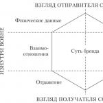 Communication strategy for brand promotion Communication brand idea
 Components of training - 稽古【Keiko】
 Role, style and way of consumption
 Customer and Contractor - relationships as the basis for the success of the project
 Encyclopedia of Marketing The main stages of marketing research